In a world awash with data, simply having numbers isn't enough. We need to make sense of them, to coax stories and insights from their raw forms. While sophisticated software can whip up intricate graphs at the click of a button, there's a unique power—and a deeper understanding—that comes from Creating Stem and Leaf Plots Manually. It's a fundamental skill, a way to truly connect with your data, revealing its shape, spread, and underlying patterns without losing a single original value.
Think of it as the artisanal approach to data visualization. It’s not just about drawing a plot; it's about dissecting your numbers, understanding their anatomy, and building a clear, insightful picture with your own hands. This guide will walk you through every step, ensuring you master this elegant and practical statistical tool.
At a Glance: Your Quick Guide to Manual Stem and Leaf Plotting
- What it is: A semi-tabular graph that organizes numerical data, showing its distribution while preserving individual values.
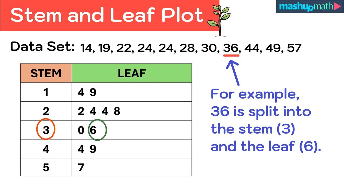
- Key components: Each data point splits into a "stem" (leading digits) and a "leaf" (the last digit).
- Why bother manually? Builds deeper data literacy, perfect for smaller datasets, quick checks, and understanding the core mechanics.
- The magic: Reveals data shape, central tendency, spread, and outliers instantly.
- Essential steps: Order data, split into stems/leaves, draw the plot, and always include a clear key.
- Don't forget: Even empty stems are important for accuracy!
Beyond the Raw Numbers: Why Stem and Leaf Plots Matter
Imagine you have a list of test scores, daily temperatures, or product sales. Just looking at a jumble of numbers often leaves you scratching your head. You might pick out the highest and lowest, but what about the overall picture? Where do most scores cluster? Are there any odd results pulling down the average?
This is precisely where the stem and leaf plot shines. It’s a clever graphical representation, sometimes called a semi-tabular tool, designed to organize and display quantitative numerical data. Unlike a histogram, which groups data into bins and loses the original values, a stem and leaf plot proudly retains every single data point. This makes it incredibly useful for understanding data distribution in detail.
By visualizing your data in this format, you can quickly identify:
- The shape of the distribution: Is it symmetrical, skewed to one side, or does it have multiple peaks?
- Central tendency: Where does most of your data fall? You can easily spot the mode (most frequent value).
- Variability (or spread): How spread out are your numbers? Are they tightly clustered or widely dispersed?
- Outliers: Are there any unusual data points that stand apart from the rest? This is critical for spotting outliers in your data that might warrant further investigation.
Ultimately, a manually crafted stem and leaf plot doesn't just present data; it invites you to explore it, making abstract numbers tangible and insightful.
Your Toolkit for Manual Plotting: Essential Prep
Before we dive into the drawing board, let's make sure you're properly equipped. Creating a stem and leaf plot manually isn't about fancy software; it's about clear thinking and methodical execution.
Gather Your Data and Get Organized
The first, and arguably most crucial, step in this manual process is to have your complete dataset ready. Whether it's written on a napkin, in a spreadsheet, or simply in your head, ensure you have all the numbers you intend to plot.
Once you have your data, the absolute non-negotiable first step is to arrange it in ascending order (from smallest to largest). This might seem tedious, especially with a larger dataset, but it’s foundational. Trying to build a stem and leaf plot with unsorted data is like trying to build a house without a foundation—it will be messy, inaccurate, and ultimately collapse.
Why is sorting so important?
- It makes identifying stems and leaves much easier and less prone to error.
- It ensures your leaves are correctly ordered next to their stems, which is a core feature of the plot.
- It allows for quick verification of your plot later (e.g., matching the minimum and maximum values).
Example Data Set (unsorted):15, 23, 12, 35, 27, 18, 23, 31, 10, 25, 30, 16
Sorted Data Set:10, 12, 15, 16, 18, 23, 23, 25, 27, 30, 31, 35
This sorted list is your blueprint. Keep it handy as we move to the next stage.
Deconstructing Your Data: Stems and Leaves Explained
The genius of a stem and leaf plot lies in its elegant simplicity: every number is split into two parts. Understanding this split is key to comparing different data sets and interpreting their underlying structure.
The Anatomy of a Data Point: Stem vs. Leaf
- The Stem: This is the leading digit or digits of your number. It represents the larger "chunks" of your data values. Think of it as the tens place, hundreds place, or even the thousands place, depending on the range of your data.
- The Leaf: This is always the last digit of your number. It represents the smaller, more granular part of your data.
Let's look at some examples to make this concrete:
| Number | Stem | Leaf |
| :----- | :--- | :--- |
| 23 | 2 | 3 |
| 15 | 1 | 5 |
| 7 | 0 | 7 |
| 152 | 15 | 2 |
| 40 | 4 | 0 |
Important Considerations for Stem/Leaf Division:
- Consistency is King: The rule for splitting must be consistent across your entire dataset. If you decide the stem is "tens" and the leaf is "ones," stick to that.
- Single-Digit Leaves: By convention, the leaf is always a single, trailing digit. If your number is 152, the leaf isn't "52"; it's "2," and the stem becomes "15." This sometimes means your stems will have multiple digits.
- Handling Single-Digit Numbers: For numbers like 7 or 9, where there's no "tens" digit, the stem is typically 0. This ensures all stems have a consistent structure relative to your data range.
A Slight Twist: Stem and Leaf Plots With Decimals
What happens when your data isn't made of neat whole numbers, but includes decimals? The logic remains remarkably similar, with just a minor adjustment to your definition of stem and leaf.
When dealing with decimal values, the stem typically represents the integer part of each number, and the leaf represents the first decimal digit.
Example Data Set (with decimals, unsorted):3.4, 2.3, 4.1, 2.7, 3.2, 2.5, 4.2, 3.5
Sorted Data Set:2.3, 2.5, 2.7, 3.2, 3.4, 3.5, 4.1, 4.2
Now, let's break these down:
| Number | Stem | Leaf |
|---|---|---|
| 2.3 | 2 | 3 |
| 2.5 | 2 | 5 |
| 2.7 | 2 | 7 |
| 3.2 | 3 | 2 |
| 3.4 | 3 | 4 |
| 3.5 | 3 | 5 |
| 4.1 | 4 | 1 |
| 4.2 | 4 | 2 |
| Notice how the stem captures the whole number, and the leaf captures the first digit after the decimal point. If you have data with two decimal places (e.g., 2.34), you'd typically round to one decimal place for the leaf, or adjust your stem to include the first decimal, and the leaf the second. However, for most basic stem and leaf plots, one decimal place for the leaf is the standard. |
The Step-by-Step Guide to Creating Your Plot Manually
Now, let's get down to the actual construction. We'll use our first sorted integer dataset as our running example:10, 12, 15, 16, 18, 23, 23, 25, 27, 30, 31, 35
Step 1: Organize Your Data (Again, Because It's That Important!)
Ensure your data is in ascending numerical order. If you skipped this step, go back and do it now. This is the bedrock of a well-formed stem and leaf plot.
Step 2: Define and List Your Stems
Look at your sorted data and identify the range of your stems. What are the lowest and highest leading digits?
- In our example:
10, 12, 15, 16, 18, 23, 23, 25, 27, 30, 31, 35 - The numbers range from 10 to 35.
- The stems will be 1 (for the 10s), 2 (for the 20s), and 3 (for the 30s).
Now, write these stems in a vertical column, from smallest to largest, with a vertical line drawn to their right. It's crucial to include all potential stems within your data's range, even if some have no corresponding leaves. This helps illustrate gaps in your data.
Stems
1 |
2 |
3 |
Step 3: Extract and Assign Your Leaves
Go through your sorted data, number by number. For each number, identify its leaf (the last digit) and write it horizontally next to its corresponding stem.
10: Stem 1, Leaf 0.12: Stem 1, Leaf 2.15: Stem 1, Leaf 5.16: Stem 1, Leaf 6.18: Stem 1, Leaf 8.23: Stem 2, Leaf 3.23: Stem 2, Leaf 3. (Yes, repeat leaves for duplicate values!)25: Stem 2, Leaf 5.27: Stem 2, Leaf 7.30: Stem 3, Leaf 0.31: Stem 3, Leaf 1.35: Stem 3, Leaf 5.
As you add leaves, ensure they are also written in ascending order next to their stem. Since you sorted your original data, this will usually happen naturally as you work through the list.
Step 4: Populate Your Plot with Leaves (First Pass)
Let's fill in our skeleton:
Stems
1 | 0 2 5 6 8
2 | 3 3 5 7
3 | 0 1 5
This looks good! Each leaf is a single digit, and they are ordered horizontally.
Step 5: Craft Your Key (Crucial for Clarity!)
A stem and leaf plot is incomplete and potentially misleading without a clear key. The key explains what the stems and leaves represent. It provides context and scale for your data.
For our example, a suitable key would be:Key: 1 | 0 = 10
This tells the reader that a stem of 1 combined with a leaf of 0 represents the number 10. If your data represented something specific, like "age in years," you might add "years" to your key, e.g., Key: 1 | 0 = 10 years.
Your Completed Manual Stem and Leaf Plot
Stems
1 | 0 2 5 6 8
2 | 3 3 5 7
3 | 0 1 5
Key: 1 | 0 = 10
Voila! You’ve manually created a stem and leaf plot. Notice how the shape of the data immediately becomes visible. You can see a cluster in the teens and twenties, with fewer values in the thirties. There are no obvious outliers, and the distribution appears relatively symmetrical around the 20s.
Example with Decimals: Putting It into Practice
Let's apply the steps to our decimal data:2.3, 2.5, 2.7, 3.2, 3.4, 3.5, 4.1, 4.2
- Organize Data: Already done (sorted above).
- Define Stems:
- Numbers range from 2.3 to 4.2.
- Stems: 2, 3, 4.
- Vertical column:
Stems
2 |
3 |
4 |
3. Extract Leaves:
- For 2.3, 2.5, 2.7: Leaves are 3, 5, 7 for Stem 2.
- For 3.2, 3.4, 3.5: Leaves are 2, 4, 5 for Stem 3.
- For 4.1, 4.2: Leaves are 1, 2 for Stem 4.
- Populate Plot:
Stems
2 | 3 5 7
3 | 2 4 5
4 | 1 2
5. Craft Key:Key: 2 | 3 = 2.3
Your Completed Decimal Stem and Leaf Plot
Stems
2 | 3 5 7
3 | 2 4 5
4 | 1 2
Key: 2 | 3 = 2.3
Now you have a clear visualization of your decimal data, showing its spread and clustering. This is a very effective way to begin uncovering central tendency and understand your dataset's shape.
Reading Your Masterpiece: Unlocking the Insights
Creating the plot is one thing; interpreting it is where the real magic happens. A stem and leaf plot is designed for quick visual analysis, allowing you to glean significant insights about your data's characteristics.
Deciphering the Plot's Language
To read any data value from your plot, simply combine a stem with one of its corresponding leaves.
- If you see
Stem: 2 | Leaves: 3 5 7and your key says2 | 3 = 23, then the data points are 23, 25, and 27. - If your key says
2 | 3 = 2.3, then the data points are 2.3, 2.5, and 2.7.
Beyond individual values, observe the overall picture:
- Shape of the Distribution: Turn the plot on its side (or imagine rotating it 90 degrees counter-clockwise). The length of each row of leaves gives you an idea of frequency. Does it look like a bell curve? Is it skewed (more data on one side)? Are there multiple peaks (bimodal)?
- Central Tendency: Where are the longest rows of leaves? This indicates where the data is most concentrated. The most frequent leaf within a stem, or the longest row of leaves, highlights the mode (most common value).
- Spread/Variability: How long are the rows of leaves, and how many stems are used? A wide range of stems and long rows indicates greater variability.
- Outliers: Are there any stems with only a few leaves that are far removed from the main body of data? Or even just a single leaf far out on a stem? These could be outliers.
- Gaps: Stems that appear in your vertical list but have no leaves indicate gaps in your data. For instance, if your data goes from the 10s to the 30s, and you included
2 |but it's empty, it means there were no values in the 20s. This is an important piece of information about your data's structure.
The beauty of manual plotting is that this interpretive process becomes intuitive. You've built the structure, so you naturally understand its components.
Common Pitfalls to Avoid When Plotting Manually
While straightforward, there are a few common missteps that can derail your manual stem and leaf plot. Being aware of these can save you time and ensure accuracy.
- Forgetting to Order the Data: This is the most frequent mistake. If your original dataset isn't sorted in ascending order, your leaves will not be in order, and your plot will be difficult to read and interpret correctly. Always, always start with sorted data.
- Incorrect Stem/Leaf Division:
- Not using the last digit as the leaf: Remember, the leaf is always the single, last digit. For
152, the stem is15, the leaf is2. Not1and52. - Inconsistent division: Once you define your stem (e.g., tens place), stick to it for all numbers.
- Mismanaging single-digit numbers: A number like
8should have a stem of0(e.g.,0 | 8) if other numbers have two or more digits, to maintain consistency.
- Omitting the Key: Without a key, your plot is ambiguous. Does
1 | 0mean 10, 1.0, or 100? The key provides essential context. - Not Including Empty Stems: If your data jumps from 19 to 31, the stem for '2' (20s) should still be listed, even if it has no leaves (
2 |). This visually represents a gap in the data, which is an important characteristic of its distribution. Ignoring empty stems can distort the visual representation of spread. - Handling Duplicate Values Incorrectly: If you have multiple instances of the same number (e.g.,
23, 23, 23), each instance must have its own leaf entry (2 | 3 3 3). Do not just list the leaf once. - Misinterpreting Decimals: Ensure your key clearly reflects how decimals are handled. If your key states
2 | 3 = 2.3, make sure you're consistent, and that you haven't accidentally represented2.3as23.
By paying close attention to these details, you'll produce a reliable and insightful stem and leaf plot every time.
When to Reach for a Stem and Leaf Plot (and When Not To)
Like any tool, the stem and leaf plot has its ideal applications and its limitations. Knowing when to use it is as important as knowing how to create it. It’s an excellent complementary tool, especially when considering how they differ from histograms.
Ideal Scenarios for Stem and Leaf Plots:
- Small to Medium Datasets (typically 15-100 values): This is where they truly shine. With too few points, they aren't very informative; with too many, they become cumbersome to create manually and difficult to read.
- Quick Visual Inspections: When you need a fast, back-of-the-envelope visualization to understand data distribution without complex software.
- Retaining Original Data: If the exact values are important for further analysis or reporting, a stem and leaf plot is superior to a histogram because no data is lost.
- Identifying the Mode: The mode (most frequent value) is often very easy to spot by looking for the most repeated leaf or the longest row of leaves.
- Comparing Two Datasets: You can create "back-to-back" stem and leaf plots to visually compare two related groups of data (e.g., test scores from two different classes). This involves sharing a central stem column, with leaves branching off to the left and right.
- Exploratory Data Analysis: It's a fantastic first step in data analysis, providing initial insights into shape, spread, and outliers before moving to more advanced statistical tests.
Limitations and When to Consider Alternatives:
- Very Large Datasets: If you have hundreds or thousands of data points, manually creating a stem and leaf plot becomes impractical and the resulting plot will be overly long and difficult to scan.
- Complex Distributions: While good for basic shapes, highly complex or multi-modal distributions might be better represented by histograms or density plots.
- Grouped Data: If your data is already grouped into classes or bins, a histogram might be a more direct visualization.
- Presentation to Broad Audiences: While informative, stem and leaf plots aren't always as visually intuitive or aesthetically pleasing for general audiences as a bar chart or histogram, which might be more familiar.
For those times when a manual plot is too much, or you need to process vast amounts of data, remember that digital tools can provide a helping hand. For those moments, you can easily Generate stem and leaf plots using online tools or spreadsheet software.
Beyond the Pencil and Paper: What About Digital Tools?
While this guide champions the manual approach for its unique learning benefits, it’s worth acknowledging that digital tools also have their place. Spreadsheet programs like Excel or Google Sheets, and specialized statistical software, can generate stem and leaf plots quickly, especially for larger datasets where manual entry becomes prohibitive.
These tools handle the sorting, stem/leaf division, and plotting with precision. However, understanding the manual process first gives you a critical edge: you understand how the software is working, you can troubleshoot issues, and you can critically evaluate the output. Without the foundational knowledge of Creating Stem and Leaf Plots Manually, you're just clicking buttons without truly understanding the statistical story they tell.
Solidifying Your Data Literacy: Next Steps in Visualization
You’ve mastered the art of creating stem and leaf plots manually, transforming raw numbers into insightful visual narratives. This isn't just a party trick; it's a foundational skill that deepens your understanding of data. You've seen how simplicity can yield profound insights, revealing the shape and spread of your data points at a glance.
Continue to practice with different datasets—try varying ranges, numbers with different decimal places, or even data with significant outliers. The more you engage with the manual process, the more intuitive data visualization will become. This skill transcends mere graphing; it cultivates a critical eye for numerical information, empowering you to ask better questions and draw more informed conclusions. Keep exploring, keep questioning, and keep making your data tell its story.